Lab 5: Learning Continuous Valued Functions
Thus far, the functions we have learned have been discrete. Each pattern was simply different from the others, and there was no meaningful way of ordering patterns. We now turn our attention to the rather more interesting task of learning a continuously valued function.

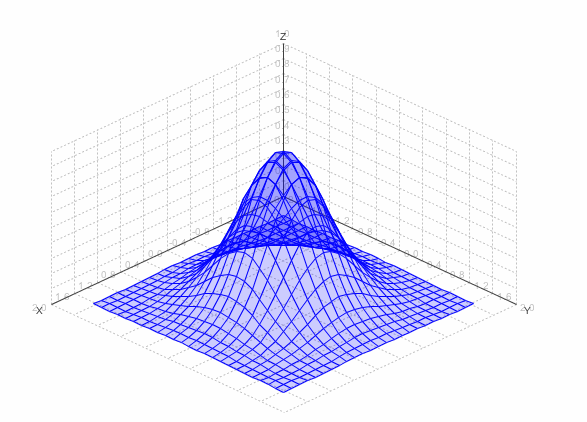
The above figure shows a simple function: the bivariate-normal function to be precise (a normal distribution in 2 dimensions). The patterns for this function are in "biNormFull.pat". Load those and create a 2-10-1 network. You can view the function you are training the network to learn by using "Utilities→3D Plotting". Make sure you choose "Target 1" as the Z (vertical) dimension.
Train the network. This may take some trial and effort. Use the same analysis function to view the network's view of the function, by repeating the above by choosing "Output 1" instead of "Target 1" as the Z-dimension of the plot. Examine both successful and unsuccessful networks.
There are two additional data sets that are derived from the same underlying function. The first, biNormNoise.pat, is similar to the one you just used, but some noise has been added. The second, biNormSparse.pat, is similar, but is much sparser (less points). See if you can get a network to learn both of these too.
In both cases, the training set is a noisy, or impure, representation of the "actual" underlying function (the bi-variate normal function). In the network outputs, can you see the underlying function? In your opinion, does the network overfit the data (i.e. model the noise)?
Try optimizing the number of hidden units used for these tasks.
For a real challenge, try learning the function found in "sinc.pat". I have not been able to get a network to learn this, but I am not 100% sure it is impossible.
