
Lab 1: Getting Started
This is the first in a series of labs. In every lab, you are encouraged to experiment, fiddle, and explore. Feel free to go beyond the suggestions made to you. At the end of each lab, if you have any feedback about what you found useful, or unhelpful, or confusing, or startling, please send me (fred.cummins@ucd.ie) a brief email about it. This feedback will help me in tuning the labs for future years.
We start with some paper and pencil exercises. In this lab, we will be looking at the basic computations done in a typical neural network. Our examples will be representative of a large class of neural networks, but will not by any means be exhaustive.
When doing this lab (and all subsequent labs), please make a note of any problems you encounter, or points you would like cleared up. We will review each lab at the start of the following lecture, and your feedback would be most welcome.
Know what is being computed
Consider this little network. The straight line in the output unit is a shorthand, meaning "this is a linear unit", or, equivalently, the net input to this unit is the same as its activation.
- Given an input of y, write down a symbolic expression for the activation of the output unit.
- Typically, all units in a network (except the input units) will have a bias unit. What role does it play in the computation here?
- What is the activation of unit 2 for the following sets of inputs and weights:
| Input | w21 | w20 | Output |
|---|---|---|---|
| 0.5 | 0.75 | -0.4 | |
| -0.5 | 0.75 | 0.4 | |
| 0 | 0.75 | 0.4 |
Simple non-linear network
Linear activation functions greatly limit the kind of input-output mapping which a network can learn (more on this later). Typically, then a unit’s activation is taken to be some function of its net input. Many popular functions are sigmoidal in shape, such as the logistic function and the hyperbolic tangent function (tanh) plotted below. In your textbook, and many simulations, you will only find the logistic function mentioned, but it is not better than other S-shaped functions, and in some circumstances alternatives, such as tanh, are to be preferred. For reasons of simplicity, our simulation software will use the logistic activation function only.
| Logistic | y=1/(1+e-x) | 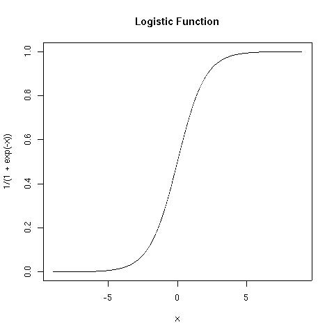 (Figure
2) (Figure
2) | |
|---|---|---|---|
| tanh | y=tanh(x) |  (Figure 3) (Figure 3) |
These are both sigmoidal (S-shaped) functions. What is the main difference between these two?
If Unit 2 in the above network had a logistic activation function, what would its output for each of the three values above be? You will need a scientific calculator or similar to compute these.
In the figure below you see a network with 5 units. The two units of the hidden layer have tanh activation functions, while the output unit is a linear unit. Unit 0 is a bias unit and is not shown (by convention) but can be assumed to have connections to units 3, 4 and 5. You should be able to write an explicit expression to describe the net input and the activation of each unit. Remember the convention that the first index of a weight is where weight leads to, and the second index is where the weight is coming from.
- If we provide inputs of 0.5 on each of units 1 and 2, what is the output at unit 5?
Some notes on software
There are several software packages out there for implementing neural network models. Some of these are large, powerful programs that allow fine-grained control over many aspects of many models. While powerful, such programs can be daunting to the inexperienced programmer. Examples of such major platforms are:
- JNNS: Java Neural Network Simulator
- Emergent: third generation platofrm developed from PDP and PDP++
- Genesis: suitable for detailed modeling of neurons
Matlab also provides a dedicated neural network toolbox that many modellers find useful. Most active researchers probably write at least some of their own code.
Then there is software for learning. When the class textbook came out, an accompanying software package called tLearn was released which served nicely to illustrate the points raised in the text. Unfortunately, that was over 10 years ago, and tLearn has not aged well. A new self-proclaimed successor to tLearn has recently emerged: called Oxlearn, it makes use of the Matlab toolbox alluded to above, although there is a stand-alone executable for Windows XP machines.
Another emerging platform that aims at supporting intuitive modelling, without programming, is Simbrain. It is still under development. Expect Simbrain 3.0 some time in 2012.
We will use a customized program that is based on an applet made by some nice German students back in 2001. The code is being rewritten for this course. Version one of the program is ready, and should run out of the box on any reasonably modern laptop.
The Basic Prop program has its own website. Go there and download the program and the pattern files you will find on the install page. The website is basicprop.wordpress.com. Put the program and the pattern files in a dedicated folder. To start the application, just double click on the icon.
When the application starts, it will look something like this:
The default network you see is a 2-2-1 network (2 inputs, one output, and a 2-unit hidden layer). Before it can do anything, use the "Patterns" menu to load in the patterns in the file "AND.pat". Examine the patterns using the checkbox in the right hand panel (the control panel). Hit "train". Now have fun. We will get to know the programme better over the coming weeks. For now, play around. Let me know what breaks it, as I want to ensure it is reasonably robust.